Page 57 - SUSTAINABILITY ISSUES & COVID-19

dependent variables used is solely the cost of debt (COD) to shed some light on the relationship between COD and ESG
disclosure. Hence, the test is not extended to YTM and EIR.

4. RESULT AND ANALYSIS

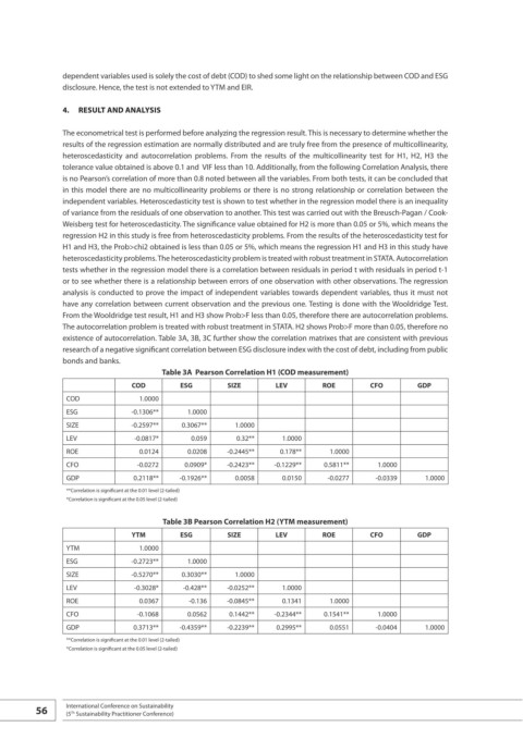
The econometrical test is performed before analyzing the regression result. This is necessary to determine whether the
results of the regression estimation are normally distributed and are truly free from the presence of multicollinearity,
heteroscedasticity and autocorrelation problems. From the results of the multicollinearity test for H1, H2, H3 the
tolerance value obtained is above 0.1 and VIF less than 10. Additionally, from the following Correlation Analysis, there
is no Pearson’s correlation of more than 0.8 noted between all the variables. From both tests, it can be concluded that
in this model there are no multicollinearity problems or there is no strong relationship or correlation between the
independent variables. Heteroscedasticity test is shown to test whether in the regression model there is an inequality
of variance from the residuals of one observation to another. This test was carried out with the Breusch-Pagan / Cook-
Weisberg test for heteroscedasticity. The significance value obtained for H2 is more than 0.05 or 5%, which means the
regression H2 in this study is free from heteroscedasticity problems. From the results of the heteroscedasticity test for
H1 and H3, the Prob>chi2 obtained is less than 0.05 or 5%, which means the regression H1 and H3 in this study have
heteroscedasticity problems. The heteroscedasticity problem is treated with robust treatment in STATA. Autocorrelation
tests whether in the regression model there is a correlation between residuals in period t with residuals in period t-1
or to see whether there is a relationship between errors of one observation with other observations. The regression
analysis is conducted to prove the impact of independent variables towards dependent variables, thus it must not
have any correlation between current observation and the previous one. Testing is done with the Wooldridge Test.
From the Wooldridge test result, H1 and H3 show Prob>F less than 0.05, therefore there are autocorrelation problems.
The autocorrelation problem is treated with robust treatment in STATA. H2 shows Prob>F more than 0.05, therefore no
existence of autocorrelation. Table 3A, 3B, 3C further show the correlation matrixes that are consistent with previous
research of a negative significant correlation between ESG disclosure index with the cost of debt, including from public
bonds and banks.
Table 3A Pearson Correlation H1 (COD measurement)
COD ESG SIZE LEV ROE CFO GDP
COD 1.0000
ESG -0.1306** 1.0000
SIZE -0.2597** 0.3067** 1.0000
LEV -0.0817* 0.059 0.32** 1.0000
ROE 0.0124 0.0208 -0.2445** 0.178** 1.0000
CFO -0.0272 0.0909* -0.2423** -0.1229** 0.5811** 1.0000
GDP 0.2118** -0.1926** 0.0058 0.0150 -0.0277 -0.0339 1.0000
**Correlation is significant at the 0.01 level (2-tailed)
*Correlation is significant at the 0.05 level (2-tailed)

Table 3B Pearson Correlation H2 (YTM measurement)
YTM ESG SIZE LEV ROE CFO GDP
YTM 1.0000
ESG -0.2723** 1.0000
SIZE -0.5270** 0.3030** 1.0000
LEV -0.3028* -0.428** -0.0252** 1.0000
ROE 0.0367 -0.136 -0.0845** 0.1341 1.0000
CFO -0.1068 0.0562 0.1442** -0.2344** 0.1541** 1.0000
GDP 0.3713** -0.4359** -0.2239** 0.2995** 0.0551 -0.0404 1.0000
**Correlation is significant at the 0.01 level (2-tailed)
*Correlation is significant at the 0.05 level (2-tailed)

56 International Conference on Sustainability
(5 Sustainability Practitioner Conference)
Th